从公式到一首歌:用代码和数学合成音乐 From Formula to Song: Making Music with Code and Mathematics

打开一段 WAV,里面没有钢琴、鼓或人声,只有一长列介于 −1 和 1 之间的数字。播放器以固定速度读出这些数字,扬声器的振膜跟着前后移动,声音就出现了。
这件事听起来很朴素,却是用代码做音乐最重要的起点:代码不需要模仿一件乐器的外观,只需要算出它随时间产生的压力变化。 音高是重复得多快,音色是一次重复里有多少层次,演奏感则藏在起音、衰减和毫秒级的偏移里。
Hitone 就按这个思路工作。它没有采样包,也不调用软音源;每件“乐器”都是 NumPy 数组上的运算。下面从一个正弦波开始,逐层走到可以导出的完整编曲。页面里的三个演示也会在浏览器里实时计算声音,点击播放时才会启动音频。
声音首先是一组采样
数字音频把连续时间切成等距的小格。采样率 Fₛ = 44100 表示每秒保存 44,100 个数。第 n 个采样发生在 t = n / Fₛ 秒;反过来,一段 T 秒的声音需要 N = T · Fₛ 个采样。
正弦波可以直接写成:
import numpy as np

SR = 44_100

def sine(freq, seconds):
    n = int(seconds * SR)
    step = 2 * np.pi * freq / SR
    phase = np.cumsum(np.full(n, step))
return np.sin(phase)固定频率时,2πft 和累计相位没有区别;一旦加入滑音或颤音,累计就很重要。频率是“这一刻相位走多快”,不是把一个不断变化的数字直接乘上时间。后者会让相位在参数改变时跳一下,耳朵听到的就是咔哒声。
固定观察窗里出现的周期越多,频率越高。波形改变了每个周期的形状,也就改变了音色。
音符名只是频率的另一种写法
十二平均律把一个八度均分成 12 份。频率每升一个八度翻倍,所以每升一个半音要乘 2^(1/12)。以 A4 = 440 Hz、MIDI 编号 69 为基准:
def frequency(midi_note):
    return 440.0 * 2 ** ((midi_note - 69) / 12)

frequency(69)  # A4  -> 440.0 Hz
frequency(72)  # C5  -> 523.25 Hz
frequency(81)  # A5  -> 880.0 Hz
因此移调不需要另一套音频。把所有频率乘 2^(n/12) 就能整体移动 n 个半音。音阶与和弦也只是半音间隔的集合:大三和弦是 [0, 4, 7],小三和弦是 [0, 3, 7]。代码保存的是关系,不是一张容易写错的频率表。
谐波决定“是什么声音”
纯正弦波只有一个频率,听起来干净,也有些空。现实里的弦、簧片和声带会同时振动出基频整数倍的成分。把它们叠加起来,就得到更复杂的周期波形:
def additive(freq, seconds, amplitudes):
    n = int(seconds * SR)
    t = np.arange(n) / SR
    out = np.zeros(n)

    for k, amp in enumerate(amplitudes, start=1):
        out += amp * np.sin(2 * np.pi * k * freq * t)

    return out / max(1, np.abs(out).max())
锯齿波的谐波大致按 1/k 下降;方波只保留奇数谐波;三角波的奇数谐波按 1/k² 很快变弱。波形名称并不神秘,它只是对一组谐波比例的简称。
点击每根谐波柱可以改变它的强度。同一个基频不动,声音仍会从柔和变得明亮、尖锐或空心。
包络让波形变成一次演奏
持续不变的波形只是测试音。钢琴、拨弦和鼓之所以容易分辨,很大一部分原因在于能量怎样进入、停留和离开。最简单的做法是给波形乘上一条包络:
def envelope(n, attack=0.005, decay=0.6, curve=2.2):
    e = np.ones(n)
    na = min(n, int(attack * SR))
    nd = min(n - na, int(decay * SR))

    e[:na] = np.linspace(0, 1, na) ** 1.3
    e[n - nd:] = np.linspace(1, 0, nd) ** curve
    return e

note = sine(220, 1.2)
note *= envelope(len(note), attack=0.004, decay=0.9)
这里故意没有使用直线衰减。被敲击或拨动的物体会在开头释放最多能量,随后越来越慢;幂曲线比一条匀速下降的直线更接近这种感觉。再进一步,Karplus–Strong 拨弦会把低通放进反馈回路,让高频先于低频消失。那种“弦在慢慢变暗”的过程,单纯把所有频率一起调小是做不出来的。
滤波器是声音与另一段数字的卷积
滤波常被画成一个旋钮,但代码真正需要的是它的冲激响应 h[n]。输入 x[n] 与 h[n] 卷积,就得到输出:
一阶低通的响应有闭式答案。设截止频率为 f:
def lowpass(x, hz):
    a = np.exp(-2 * np.pi * hz / SR)
    length = int(np.log(1e-4) / np.log(a))  # 衰减到 −80 dB
    h = (1 - a) * a ** np.arange(length)
    return np.convolve(x, h)[:len(x)]
这段实现没有逐采样更新滤波器状态,而是先把公式一次写成数组,再交给卷积。短响应直接卷积,长响应改用 FFT。两种算法在听感上没有区别,却会决定一首几分钟的曲子是数秒还是数分钟才能重新生成。渲染越快,参数才真的改得动。
节奏是把音乐时间换算成采样位置
编曲最好不要直接写秒数。120 BPM 时一拍是 0.5 秒;改成 96 BPM 后,散落在代码里的 1.0、1.5 和 2.0 不会自己排回小节。稳定的接口应该接收小节与拍:
class Track:
    def __init__(self, bpm=120, swing=0.5):
        self.bpm = bpm
        self.beat = 60.0 / bpm
        self.bar_seconds = 4 * self.beat
        self.swing = swing

    def at(self, bar, beat=0.0):
        whole, fraction = divmod(float(beat), 1.0)
        if abs(fraction - 0.5) < 1e-9:
            fraction = self.swing
        return bar * self.bar_seconds + (whole + fraction) * self.beat
Swing 也只应该在这里处理一次。把半拍从 0.50 推到 0.58,所有踩镲、贝斯和侧链包络都会遵守同一个时间网格,不会出现鼓已经摇摆、其他声部还走直线的情况。
开启或关闭十六分音符,再改变 BPM 和 Swing。圆点的位置来自同一个 at() 公式,播放缓冲区也按这些位置生成。
从音符到一首歌,需要分层而不是堆叠
声音函数解决“一个音怎样响”,编曲解决“它何时出现”。两层不要混在一起。下面这段只谈小节、和弦与力度,不关心电钢琴内部用了几层 FM:
t = Track(bpm=104, bars=32, swing=0.56)
t.bus('keys', send=0.18, chorus={'rate': 0.42}, width=13)

progression = ['Amaj7', 'F#m7', 'Dmaj7', 'Eadd9']
for bar in range(32):
    chord = progression[bar % len(progression)]
    for freq in ch(chord, octave=3):
        note = rhodes(freq, at(1.8)) * envelope(at(1.8))
        t.add('keys', note, t.at(bar, 0), gain=0.22)
每个声部先进入自己的 bus,再统一处理声像、合唱、延迟、混响和侧链。混音的本质仍是加法:对齐时间后把数组相加。需要注意的只有余量——多个不削波的声部叠在一起仍可能超过 [-1, 1]。总线留出空间,母带末端再做轻微软削波和峰值归一化,比每放一个音就偷偷压小要清楚得多。
最后一步不是“听起来应该没问题”
代码生成的声音可以被重复验证。相同随机种子应当得到完全相同的文件;BPM 可以从实际音频重新测量;每个段落的 RMS、峰值和频谱重心也都可以计算。频谱图尤其有用,因为它能把整首曲子的结构压在一张图里。
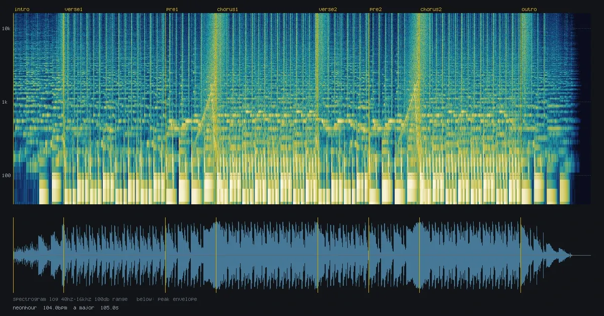
这不是装饰图。横轴是时间,纵轴是对数频率,亮度是能量;下方曲线记录峰值包络。主歌是否过满、低频是否中途消失、渐强有没有真的发生,都能直接看见。
到这里,一首歌仍然只是数字,但这些数字已经有了清楚的来源:频率给出音高,谐波给出音色,包络与滤波塑造动作,时间网格组织节奏,bus 和母带把它们放进同一个空间。代码保存的不只是最后的 WAV,也保存了这首歌为什么会这样响。
完整的合成器、编曲和分析工具可以在 Hitone 源码 中查看。
Open a WAV file and there is no piano, drum, or voice inside. There is only a long column of numbers between −1 and 1. A player reads them at a fixed rate, the loudspeaker cone follows their movement, and sound appears.
That plain fact is the useful starting point for making music in code: the program does not have to imitate what an instrument looks like. It only has to calculate the pressure changes that instrument would make over time. Pitch is how quickly a pattern repeats. Timbre is the detail within one repetition. Performance lives in the attack, decay, and differences of a few milliseconds.
Hitone works this way. It contains no sample packs and calls no software instruments; every “instrument” is arithmetic on a NumPy array. The sections below start with one sine wave and build toward a complete arrangement that can be written to disk. The three demos calculate their audio in the browser too, and remain silent until Play is pressed.
Sound begins as samples
Digital audio cuts continuous time into evenly spaced cells. A sample rate of Fₛ = 44100 stores 44,100 numbers per second. Sample n occurs at t = n / Fₛ seconds; in the other direction, a sound lasting T seconds needs N = T · Fₛ samples.
A sine wave can be written directly:
import numpy as np

SR = 44_100

def sine(freq, seconds):
    n = int(seconds * SR)
    step = 2 * np.pi * freq / SR
    phase = np.cumsum(np.full(n, step))
    return np.sin(phase)
At a fixed frequency, 2πft and accumulated phase give the same answer. Accumulation matters as soon as the note bends or vibrato arrives. Frequency says how quickly phase is moving now; it is not a changing number to multiply by time. The latter makes phase jump when a parameter moves, and the ear hears the jump as a click.
More cycles inside the fixed window mean a higher pitch. Changing the shape changes the detail inside each cycle, so it changes the timbre too.
A note name is another way to write a frequency
Twelve-tone equal temperament divides an octave into twelve equal ratios. Frequency doubles over an octave, so each semitone multiplies it by 2^(1/12). With A4 = 440 Hz at MIDI note 69:
def frequency(midi_note):
    return 440.0 * 2 ** ((midi_note - 69) / 12)

frequency(69)  # A4  -> 440.0 Hz
frequency(72)  # C5  -> 523.25 Hz
frequency(81)  # A5  -> 880.0 Hz
Transposition therefore needs no new audio. Multiply every frequency by 2^(n/12) to move the entire part by n semitones. Scales and chords are just collections of semitone intervals: a major triad is [0, 4, 7], a minor triad [0, 3, 7]. The code keeps the relationship rather than a frequency table where a typo can hide.
Harmonics decide what the sound is
A pure sine contains one frequency. It sounds clean and a little empty. Real strings, reeds, and vocal folds vibrate at integer multiples of a fundamental at the same time. Add those components and a richer periodic shape appears:
def additive(freq, seconds, amplitudes):
    n = int(seconds * SR)
    t = np.arange(n) / SR
    out = np.zeros(n)

    for k, amp in enumerate(amplitudes, start=1):
        out += amp * np.sin(2 * np.pi * k * freq * t)

    return out / max(1, np.abs(out).max())
A sawtooth has harmonics that fall roughly as 1/k. A square keeps only odd harmonics. A triangle keeps the odd ones but lets them fall quickly as 1/k². The names are not mysterious; each is shorthand for a particular list of harmonic levels.
Click a harmonic column to change its strength. The fundamental stays fixed while the sound moves from soft to bright, sharp, or hollow.
An envelope turns a waveform into a performance
An unchanging waveform is a test tone. A piano, plucked string, and drum are easy to tell apart largely because of how their energy arrives, holds, and leaves. The smallest useful step is to multiply the waveform by an envelope:
def envelope(n, attack=0.005, decay=0.6, curve=2.2):
    e = np.ones(n)
    na = min(n, int(attack * SR))
    nd = min(n - na, int(decay * SR))

    e[:na] = np.linspace(0, 1, na) ** 1.3
    e[n - nd:] = np.linspace(1, 0, nd) ** curve
    return e

note = sine(220, 1.2)
note *= envelope(len(note), attack=0.004, decay=0.9)
The decay is deliberately not a straight line. A struck or plucked object gives up most of its energy early and then fades more slowly; a power curve is closer to that motion than a constant-rate fade. Karplus–Strong synthesis goes further by putting a lowpass inside a feedback loop, so high frequencies disappear before low ones. That gradual darkening is what a string does, and scaling all frequencies with one envelope cannot reproduce it.
A filter is convolution with another column of numbers
Filters are often drawn as knobs, but code needs their impulse response h[n]. Convolve the input x[n] with h[n] to produce the output:
A one-pole lowpass has a closed-form response. For cutoff frequency f:
def lowpass(x, hz):
    a = np.exp(-2 * np.pi * hz / SR)
    length = int(np.log(1e-4) / np.log(a))  # decay to −80 dB
    h = (1 - a) * a ** np.arange(length)
    return np.convolve(x, h)[:len(x)]
This implementation does not update filter state sample by sample. It writes the formula into an array once and hands it to convolution. Short responses use direct convolution; long responses move to an FFT. The two routes sound the same, but they decide whether a multi-minute track can be regenerated in seconds or minutes. Fast rendering is what makes parameters genuinely editable.
Rhythm converts musical time into sample positions
An arrangement should not be written directly in seconds. At 120 BPM, one beat lasts 0.5 seconds. Change the tempo to 96 and scattered values such as 1.0, 1.5, and 2.0 will not arrange themselves back into bars. A stable interface accepts bars and beats:
class Track:
    def __init__(self, bpm=120, swing=0.5):
        self.bpm = bpm
        self.beat = 60.0 / bpm
        self.bar_seconds = 4 * self.beat
        self.swing = swing

    def at(self, bar, beat=0.0):
        whole, fraction = divmod(float(beat), 1.0)
        if abs(fraction - 0.5) < 1e-9:
            fraction = self.swing
        return bar * self.bar_seconds + (whole + fraction) * self.beat
Swing belongs here too, exactly once. Push the off-eighth from 0.50 to 0.58 and every hi-hat, bass note, and sidechain envelope follows the same grid. The drums cannot swing while the rest of the arrangement continues in a straight line.
Toggle sixteenth notes, then change BPM and Swing. The circles use the same at() calculation as the generated playback buffer.
A song needs layers, not a pile of notes
Sound functions answer “how does one note speak?” Arrangement answers “when does it appear?” Keep those layers separate. This passage talks only about bars, chords, and level; it does not need to know that the electric piano uses FM internally:
t = Track(bpm=104, bars=32, swing=0.56)
t.bus('keys', send=0.18, chorus={'rate': 0.42}, width=13)

progression = ['Amaj7', 'F#m7', 'Dmaj7', 'Eadd9']
for bar in range(32):
    chord = progression[bar % len(progression)]
    for freq in ch(chord, octave=3):
        note = rhodes(freq, at(1.8)) * envelope(at(1.8))
        t.add('keys', note, t.at(bar, 0), gain=0.22)
Each part enters its own bus before panning, chorus, delay, reverb, and sidechain are applied consistently. Mixing is still addition: align the arrays in time and sum them. The remaining issue is headroom. Several parts that do not clip alone can exceed [-1, 1] together. Leaving space on the buses, then applying gentle soft clipping and peak normalisation at the master, is clearer than quietly turning down every note as it is placed.
The last step is not “it probably sounds fine”
Code-generated audio can be checked repeatedly. The same random seed should produce the same file. Tempo can be measured again from the rendered audio. RMS, peak, crest factor, and spectral balance can be calculated for each section. A spectrogram is especially useful because it compresses the whole structure into one image.
This is not decoration. Time runs across the page, logarithmic frequency rises vertically, and brightness shows energy. A crowded verse, a low end that disappears halfway through, or a crescendo that never happened becomes visible at once.
The finished piece is still a column of numbers, but every number now has a reason to be there. Frequency gives pitch, harmonics give timbre, envelopes and filters shape gestures, the time grid organises rhythm, and buses place everything in one space. The code preserves not only the final WAV, but why the piece sounds the way it does.
The complete synthesis, arrangement, and analysis code is available in the Hitone repository.